MNIST handwritten image classification with Naive Bayes and Logistic regression.

Exploring the Nave Bayes and Logistic regression classifiers, discussing the implementation of both the classifiers on the problem of classifying the MNIST dataset that contains the images of handwritten numbers. Assumption on probability of each class are made to classify the images.
I. MNIST DATASET
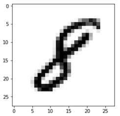
MNIST — Modified National Institute of Standards and Technology is a large database of handwritten digits from 0–9. The project uses the modified MNIST dataset with 60000 train data and 10000 test data. It is one of the most commonly used datasets for Machine Learning. Each image in both training and test set is a grey scale image of dimension 28x28 pixels. Below (fig 1.1) is an example indicating digit 8.

II. NAIVE-BAYES ALGORITHM
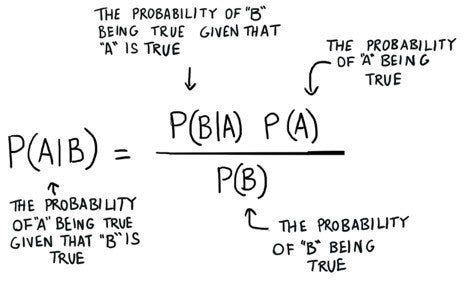
Naive — Bayes is a classifier which uses Bayes Theorem. It calculates the probability for membership of a data-point to each class and assigns the label of the class with the highest probability. Naive Bayes is one of the fastest and simple classification algorithms and is usually used as a baseline for classification problems.
III. LOGISTIC REGRESSION
The Logistic Regression is classification algorithm used when the output is categorical. The ideology behind the classification is finding the relationship between the features and probabilities. The results can be interpreted as likelihood that the data in the question belongs to a particular class.
NAIVE — BAYES CLASSIFIER.
The problem involves building a Naive Bayes classifier on MNIST dataset. Results include confusion matrix, accuracy of each digit, and over accuracy. It also assumes that probability of each pixel is a Gaussian distribution and the probability of each digit is equal.
Each image in MNIST dataset is a 28x28 pixels but for our purpose we are converting the images in a single flat array of 784 pixels. Knowing that each pixel from the array can take values between 0–255, it appears like continuous data. To ease the computation, we use Gaussian to get the probabilities of each pixel given a class.
The equation used:

The number of dimensions being very large, the probabilities obtained are very small to overcome this we take the log likelihood.

Each pixel in data is assumed to have a Gaussian distribution, the code uses Scikit Learn modules Gaussian Naive Bayes classifier, each class is assigned with equal probability. Mean and standard deviation is calculated to summarize the distribution of the data, for each class
Mean(x) = 1/n * sum(x),
where n = number of times the unique value is repeated for an input variable x.
Standard deviation (x) = √ (1/n* Σ(xi-mean(x)²)),
it is the root of squared distance of input value x from mean value of x where is n is the number of times the unique value is repeated.
To calculate the probability of new x value the Gaussian probability density function is used. The Gaussian PDF provides an estimate value of probability that x belongs to a certain class.

Observations
- Naive Bayes Classifier does not a appear to perform well for MNIST data set as it produced an overall accuracy of 56%.
- 2. Looking at confusion matrix (fig 2) below, we can observe that (5,8), (5,9), (4,8), (4,9), (7,9) are some of the combinations where the classifier is confused in predicting the right label.

We can express 784 individual Gaussian distributed as a one long string of multivariate Gaussian, we can infer from that covariance matrix Σ except the diagonal of the matrix everything else will be zeros, hence only the 784 variances are stored at the diagonal.
The downside in the Naive Bayes classifier is that it assumes the all the dimensions present in the data set is independent to one another and which we all know that it’s not correct.
After training the model, the classifier shows it has understood to label by plotting Mean (μ) of each class.
To plot the mean of each feature per class Scikit Learn Naive Bayes Gaussian module has an attribute theta_ which returns the mean of each feature of every single class.
Below are the few example graphs which represent the label which the classifier understood by obtaining the mean of each class.

The Images show the Mean and variance of the feature of each class. The images appear to take the shape of the class to which they belong.
Logistic Regression classifier:
The Problem involves building a regularized logistic regression with ridge (l2) regularization. Further the problem expects building 10 classifiers for 0 vs all, 1 vs all etc. Also demands the confusion matrix, accuracy of each digit and overall accuracy. Finally, a plot of accuracy vs regularization value where a log-scale us used on regularized value.
Logistic regression begins with the sigmoid function which is the standard logistic function. It accepts values between zero and one. Below is the sigmoid equation:

Here 𝜔0,𝜔1 .. are the logistic regression coefficients of the model and these coefficients are calculated using the maximum likelihood estimation. Sigmoid function finds the probability of the binary outcome and using the obtained probability the classes are labeled.
Role of Ridge Regularization (L2), The ridge adds the constraints to the coefficients. The Lambda value is used for the regularization, ridge regression reduces the complexity in the model by bringing the coefficients near by or shrinking it towards zero.
The L2 regularization uses the below mentioned equation i.e. the log likelihood.

One vs all Classifier:
The one vs all classifier works on the strategy of fitting one binary class per classifier. We combine all the positive examples for given class and rest are assigned to another class. For our problem we have created 10 such classifier, where each classifier takes one digit as positive and rest as negative.
After creating 10 classifiers, for instance 1 vs all classier is created to obtain the probability of the digit 1 versus for all other classes. Here, the digit 1 belongs to class +1 and all other digits are considered as class -1. Here in this method maximum probability among all the 10 classifiers are picked to provide the prediction of class of the given image.
To optimize the Logistic Regression classifier, we use gradient descent to minimize the loss. The best value for the weights W is obtained using the gradient descent. To start with, a vector of 785 (including a bias term) 0s’ is taken. We continuously update the value of weights in each iteration to the point of convergence. The weights are updated by subtracting the gradient descent times the learning rate. In our problem the learning rate is from 0.0001 to 100 with the multiples of 10.
After taking the gradient of equation 2.1 i.e., by taking the derivative of ℒ(𝑤) we get

Observations:
- Looking at confusion matrix (fig 2) below, we can observe that (2,8), (4,9), (5,3), (5,8), (7,9) are some of the combinations where the classifier is confused in predicting the right label.

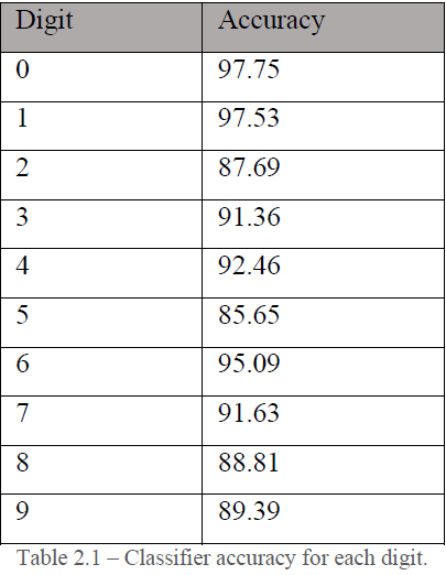
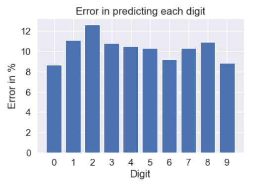
2. Accuracy of Each digit

3. Overall accuracy for different lambda values are tabulated below:


As we observe from the table 2.2 the accuracy is maximum for the lambda value 100. Also, computationally lambda=100 the classifier performs faster., But we should keep in mind to not selection of value should be dynamic in the code. The observation is only for this dataset and our model.

1. Logistic regression is more efficient than the Naive — Bayes algorithm, the overall accuracy obtained is 91.85% where in Naive — Bayes ended up 61.82% test accuracy. Logistic Regression being complex as compared to the Naive — Bayes algorithm, Logistic Regression model performed well in classifying the images.
2. Logistic Regression is more computationally expensive than Naive Bayes. The Naive Bayes took less than a minute to train and predict the labels, whereas Logistic Regression took about an hour to train and predict the labels.
3. Nave Bayes classifier assumes all the dimensions as independent to one another which is not true.
*******************************************************************
Code Snippets:
Creating a Naive Bayes Classifier
1. The function takes training features, labels and Test features as input parameters.
2. Functions calculates the mean and covariance for each label and stores it in a dictionary.
3. The Prior probabilities is obtained by taking the number of times class occured divided by sample length.
4. Using these means and covariances, calculate probability that the test input belongs to a given class.
5. From the list of probabilities for each class we pick the maximum probability to decide which class the input belongs to.
6. Plot images for mean and variances.
7. Return a list of prediction values for further calculations.
Logistic Regression Classifier
1. The first step in the logistic regression classifier is to find the optimized using the gradient decent using TNC method, iteratively optimize the values of weight.
2. We combine all the positive examples for given class and rest are assigned to another class. For our problem we have created 10 such classifier, where each classifier takes one digit as positive and rest as negative.
3. Tabulating the accuracy for each Lambda — Regularized value.
References
[1] CS5841 — Machine learning by Dr. Timoty Havens, Lecture slides.
[2] Lazy Programmers- Source of deep learning and Machine Learning.
[3] K. Elissa, “Title of paper if known,” unpublished.
[4] Logistic Regression Overview Towards Data Science..
[5] Pattern recognition and Machine Learning by Bishop.
[6] DataCamp Ridge and Lasso Regularization.
[7] Machine Learning Mastery — Naive Bayes.
